Authors:
(1) Davide Viviano, Department of Economics, Harvard University;
(2) Lihua Lei, Graduate School of Business, Stanford University;
(3) Guido Imbens, Graduate School of Business and Department of Economics, Stanford University;
(4) Brian Karrer, FAIR, Meta;
(5) Okke Schrijvers, Meta Central Applied Science;
(6) Liang Shi, Meta Central Applied Science.
Table of Links
Empirical illustration and numerical studies
3 (When) should you cluster?


3.1 Worst-case bias


3.2 Worst-case variance

Lemma 3.2 states that two realized outcomes have zero covariance if two individuals (i) are in two different clusters, such that none of the two clusters contains a friend of the other individual, and (ii) are not friends or share a common friend (set), and if there is no friend of j in a cluster that contains a friend of i (set Gi). Note that Lemma 3.2 is equivalent to saying that µi(Di , D−i)[2Di − 1], µj (Dj , D−j )[2Dj − 1] have zero covariance if Bi ∩ Bj = ∅. Next, we analyze the covariances for the remaining units.


Remark 5 (Unobserved A). Suppose that A is unobserved or partially observed, and researchers have a prior over A. In this case, the characterization of the bias and variance continue to hold once we take expectations with respect to the distribution of A, where the prior over A may depend on partial network information [e.g. Breza et al., 2020].
3.3 Comparison with a Bernoulli design


now the number of clusters is of order n (e.g., clusters contain few individuals each). Then the cluster design is optimal.
Table 1: Practical implications of Theorem 3.5. Rule of thumb is computed for λ = 1, in the presence of equally sized clusters with outcomes taking values between zero and one, and the bias of the clustering equal (or smaller than) 50% (i.e., for each individual, 50% of her connections are in her same cluster). Here ψ¯ ≤ 4 when outcomes are binary.

For λ = 1, known ψ¯, the rule of thumb provides the smallest spillover effects that would guarantee that the cluster design dominates the Bernoulli design.
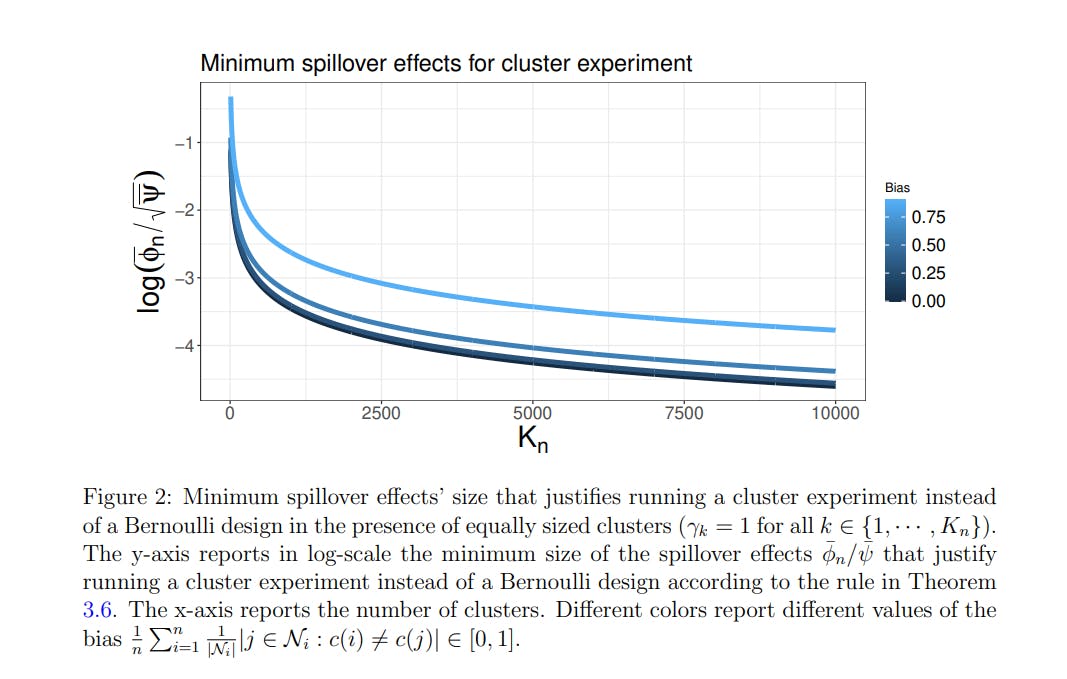
The last column in Table 1 collects the implications of the rule of thumb, assuming (i) equally sized clusters, (ii) the bias of the clustering is at most 50% as a conservative upper bound, and (iii) outcomes are bounded between zero and one (in which case ψ¯ ≤ 4). In this setting, researchers should run a cluster experiment when ϕ¯ n √ Kn is larger than 2.3 when ψ¯ = 4. Figure 2 illustrates the rule of thumb as a function of the bias and clusters.

[10] The condition Kn/n = o(1), can be relaxed by a finite sample condition Kn ≤ nδ′ (ψ/ψ¯) for some δ ′ ∈ [0, 1). In particular, under the assumptions in Section 4.2, ψ = ψ¯ and the condition is equivalent to that a fixed fraction of clusters have more than one observation.
This paper is available on arxiv under CC 1.0 license.